Summary: I built a spreadsheet model to demonstrate the impact on saving lives of implementing controls sooner rather than later to contain the spread of coronavirus. You can copy the model, edit the assumptions, and run your own scenarios.
If you're anything like me, you spent much of the weekend glued to your phone reading the latest news updates on the novel coronavirus (2019-nCoV) that causes the Covid-19 disease. Or perhaps you were nervously eyeing stock market futures (or both).
It doesn't help that cases have spiked abroad. While cases number around 500 as of March 9 in the United States, there are over 7,300 in Italy, which today expanded travel restrictions to the whole country.
It also doesn't help that official government statements about the potential impact of coronavirus in the United States are conflicting. President Trump tweeted at the end of February that the coronavirus is "very much under control in the USA."
On the other end of the spectrum, Dr. Anthony Fauci, director of the National Institute of Allergy and Infectious Diseases, told Fox News on Sunday:
You don’t want to alarm people, but given the spread we see, you know, anything is possible. And that’s the reason why we’ve got to be prepared to take whatever action is appropriate to contain and mitigate the outbreak.
Anything is possible?
The virus has spread to two-thirds of the states, with more than 20 deaths. How bad could it get? Who are we to believe?
Perhaps we don't have to simply believe. We can do our own analysis. After all, we have access to the same technology that epidemiologists use to forecast epidemics — spreadsheets!
This post is part of a series on modeling the COVID-19 impact using spreadsheets. Be sure to read the other articles in the series for the latest models and information.
- Part 1: A simple model for forecasting the impact of coronavirus and controls (March 9)
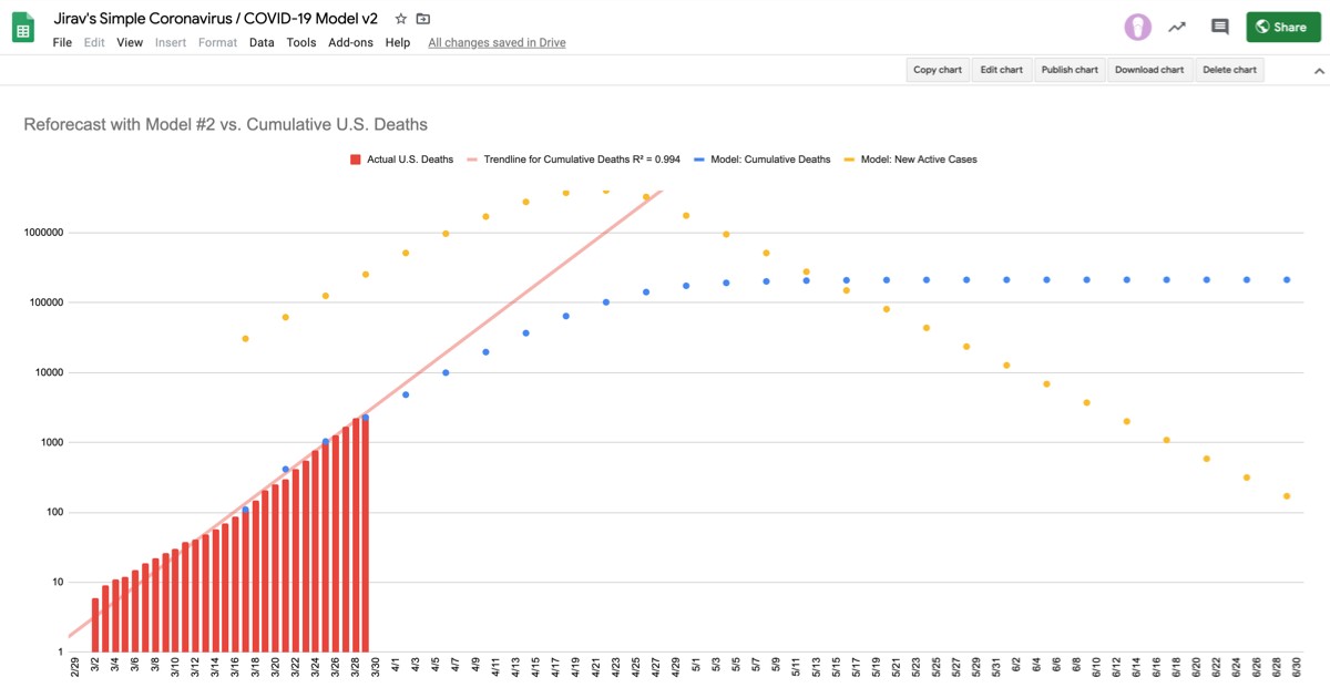
- Part 2: Reforecasting the U.S. COVID-19 Impact (March 30)
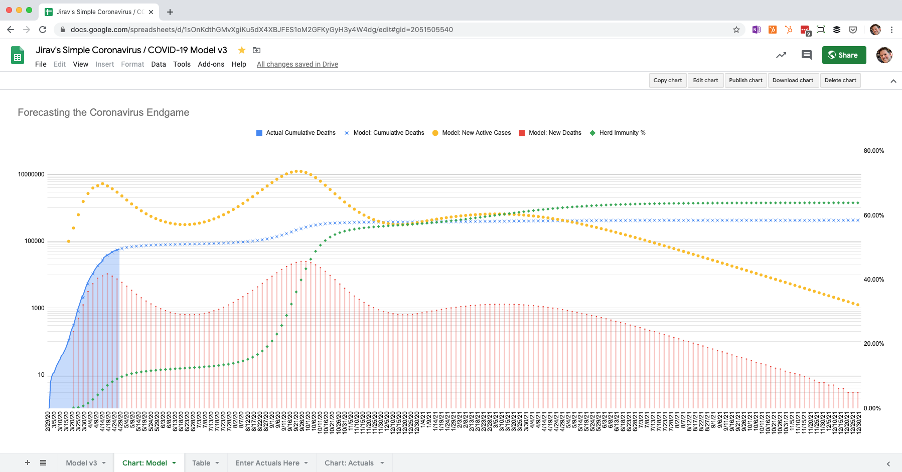
- Part 3: Forecasting the End of COVID-19: Herd Immunity (April 29)
I've been working at Jirav since October, and we make software built on top of a driver-based financial modeling engine, so I'm a bit obsessed with financial models right now.
As I was contemplating an uncertain future in a world with Covid-19 this past weekend, I realized that I could perhaps bring a bit more certainty to the world by building a model using the formulas I've been seeing crop up in the news.
At the very least it might help us understand a bit better why epidemiologists and folks working at the CDC and other health agencies seem so worried.
Our inputs and outputs in a coronavirus impact model aren't financial statements, but the same principles apply. Keep on reading to learn about the formula and how the model is built, or scroll to the bottom to download your own copy and tweak my assumptions.
The basic model for epidemiological spread
First, a disclaimer.
I am a CPA, not an epidemiologist, mathematician, or statistician. I'm proud to say that I did get an A in multivariable calculus at Northwestern University, but you should still read everything below with a healthy dose of skepticism. (And please do let me know if I made any mistakes.)
Also, the purpose of this exercise is not to frighten anyone. It is to give you information so you can make your own determination of the risks to you, your family, your business, and your customers. While creating this model has caused me to worry more about the potential consequences of inaction, I am comforted that a timely and adequate response by our leaders has the great likelihood of minimizing the impact to a much less frightening level.
Now that that's out of the way, let's continue.
Here is a (relatively) simple formula for viral growth as presented in a February 5 paper in the Annals of Internal Medicine:
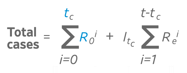
The formula looks complicated, especially if you're not familiar with summation notation, but it makes a whole lot more sense when we visualize it in a spreadsheet, so bear with me.
Basically, we're adding together the pieces of two exponential functions. If you know how to calculate exponents, you can build this model. An example of an exponential formula is 2^3 = 2 x 2 x 2 = 8. That's pretty much all we're doing here a bunch of times with different variables, then adding it all up.
Let's start with the first component of the formula:

Part 1: Uncontrolled spread
The first part of the equation represents exponential growth without control measures. The variables we need to know are R0, t, and i. The big "E" looking symbol is a sigma — it means that we are going to do this calculation one or more times and then add up our results.
R0 (pronounced "R-naught") stands for the the basic reproductive number. This is the number of people each infected person will infect in turn if there is little or no effort to quarantine infected people or otherwise keep them from infecting the rest of the population.
R0 seems to be around 2.3 according to a paper available on PubMed.gov. I've also seen estimates of 2.6 — but it probably doesn't matter much, as any value of 2 or higher will grow very quickly, as you'll see below.
The variable t represents the number of serial intervals that have passed — the upper limit of our sum. A serial interval is how long it takes on average for an infected person to spread the disease to R0 others. There are many different estimates of the serial duration from as little as 4 days to as long as 7.5 days. For our model, I went with 7 days. That means after 10 intervals (t), 70 days will have passed.
i represents where to start. For the first part of the equation, this is 0 because we are starting at the beginning.
Knowing R0, t, and i, all we have to do now is calculate the function for each interval in the range, and then add up our results to get the total number of cases.
Here's an example:
Let's assume that the virus spreads for 5 serial intervals (35 days) without control. We have to calculate R0^i for the values R0=2.3 and i from 0 to 10.
2.3^0 = 12.3^1 = 2.32.3^2 = 5.292.3^3 = 12.172.3^4 = 27.982.3^5 = 64.36
Add up the results (1 + 2.3 + 5.29 +12.17 + 27.98 + 64.36), round to the nearest integer, and we get 112 cases. It's very easy to model this out in a spreadsheet — it's just a bunch of multiplication and addition.
Here's what that looks like:

You may have noticed how quickly the number of infected increases. That's because R0 (the basic reproductive rate) is greater than 2. The result more than doubles each interval. In this case, by day 56 of the outbreak the total number of infected has already reached 1,374, and will continue doubling.
This leads to some potentially frightening outcomes. If the coronavirus is not contained, and assuming that the serial interval is 7 days, in just under 100 days, over 200,000 people could become infected.
But don't worry too much yet — we have to add in the second part of the equation, when we start implementing controls to reduce the spread.
Part 2: Controls implemented
The second part of the function is much the same as the first.
The difference is the value of R, now Re, known as the effective reproduction rate. This number should be lower than R0 due to the introduction of control measures such as testing, quarantines, and perhaps even the invention of a vaccine.
To calculate the total number of cases, we continue our model in spreadsheet form, but we lower the value of R. I'm going with 1.5 based on the model published in the Annals of Internal Medicine in February.
In other words, by reducing R from 2.3. to 1.5 the control measures implemented so far in impacted areas of the world have reduced the reproductive rate by about 35%.

Building out the spreadsheet model
Once we know the number of infected, we can begin to project the number of deaths. As with all the variables, the case fatality rate is uncertain. Estimates from studies and news reports available online range from as high as 3.4% and as low as .7%. For my model, I've gone with 1% for now.
For simplicity, I've also assumed that new deaths occur two intervals after a case develops. If the interval is 7 days, that means an infected person has a 1% chance of dying 14 days later.
Now we can model out the first 100 or so days of the virus given three scenarios:
- Scenario 1: Uncontrolled spread
- Scenario 2: Late implementation of controls (after ~100 deaths are reported)
- Scenario 3: Early implementation of controls (after ~10 deaths are reported)
The results are dramatic:
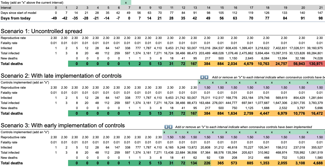
Under Scenario 1, the contagion spreads rapidly within 100 days of the first death to infect 69 million people, killing 131,000 at this point.
Under Scenario 2, controls are implemented after deaths exceed 100. In the same 100 days, 3.8 million become infected and 16,472 have died 100 days after the first death.
Under Scenario 3, controls are implemented as soon as deaths exceed 10. Only 1 million people are infected and 4,688 have died 100 days after the first death.
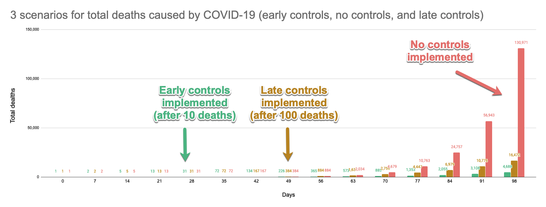
A chart helps to illustrate the impact of controls on saving lives:
Conclusions
The difference between early and late implementation of controls is only 3 weeks in this model, but it makes an enormous difference. It dramatically reduces the spread of the virus, and also buys time to work on reducing the reproductive number below 1 (at which point the virus will die out, since each infected person will infect fewer than 1 other person, on average). Obviously, failing to take any action is catastrophic. And it is far better to act sooner rather than later.
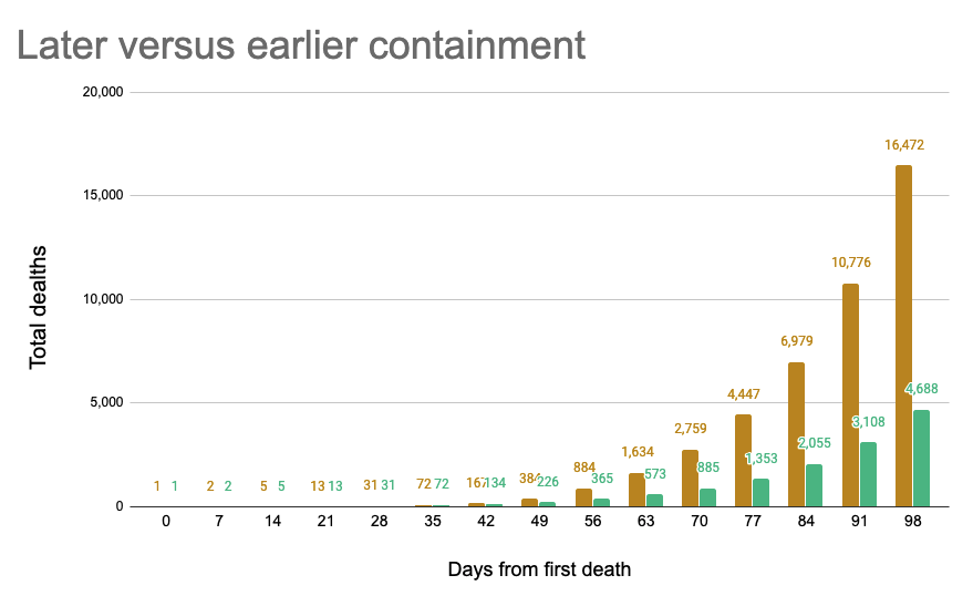
Implementing controls 3 weeks earlier saves 11,784 lives by the 98 day mark.
The challenge is knowing when to act. Implementing controls such as universal testing, mandatory quarantines, and travel restrictions is difficult, disruptive to citizens' lives, and harmful to the economy. Leaders may hesitate to take drastic action and what seems like a low level of cases and deaths. But every week that passes significantly reduces the ultimate effectiveness of containment efforts.
Limitations of the model — and what it does well
This is about the simplest way to calculate the spread of a disease possible. Therefore it has many limitations. The model doesn't account for the variety of ways in which individuals, businesses, and the government may implement controls and the varying effectiveness of those controls. It doesn't account for possible mutation of the virus. It doesn't account for geographic boundaries. It doesn't account for variation in the population when it comes to natural immunity or other factors.
However, the model does illustrate very well how quickly a highly contagious virus can spread and get out of control. Anything that can be represented by an exponential function can be hard to grasp since we don't often encounter exponential natural phenomena in our daily lives. We're much more accustomed to linear growth.
Download the model and forecast using your own assumptions
View my model in Google Sheets. You can also download your own copy in Excel format:
Change the assumptions in your own copy to see what happens. I hope you find it helpful in understanding the potential impact of the coronavirus. Let me know your thoughts and/or feedback in the comments below, and be sure to wash your hands!
If you want to use this model to drive a forecast for your business, you could even build it out as part of Jirav's budgeting and planning software. For instance, you could use the percentage of the population infected to drive the proportion of your company's team that will be out sick, or the impact on sales. If you're interested in learning how to do that, request a demo and we'll be happy to show you how it works.






.jpg)

